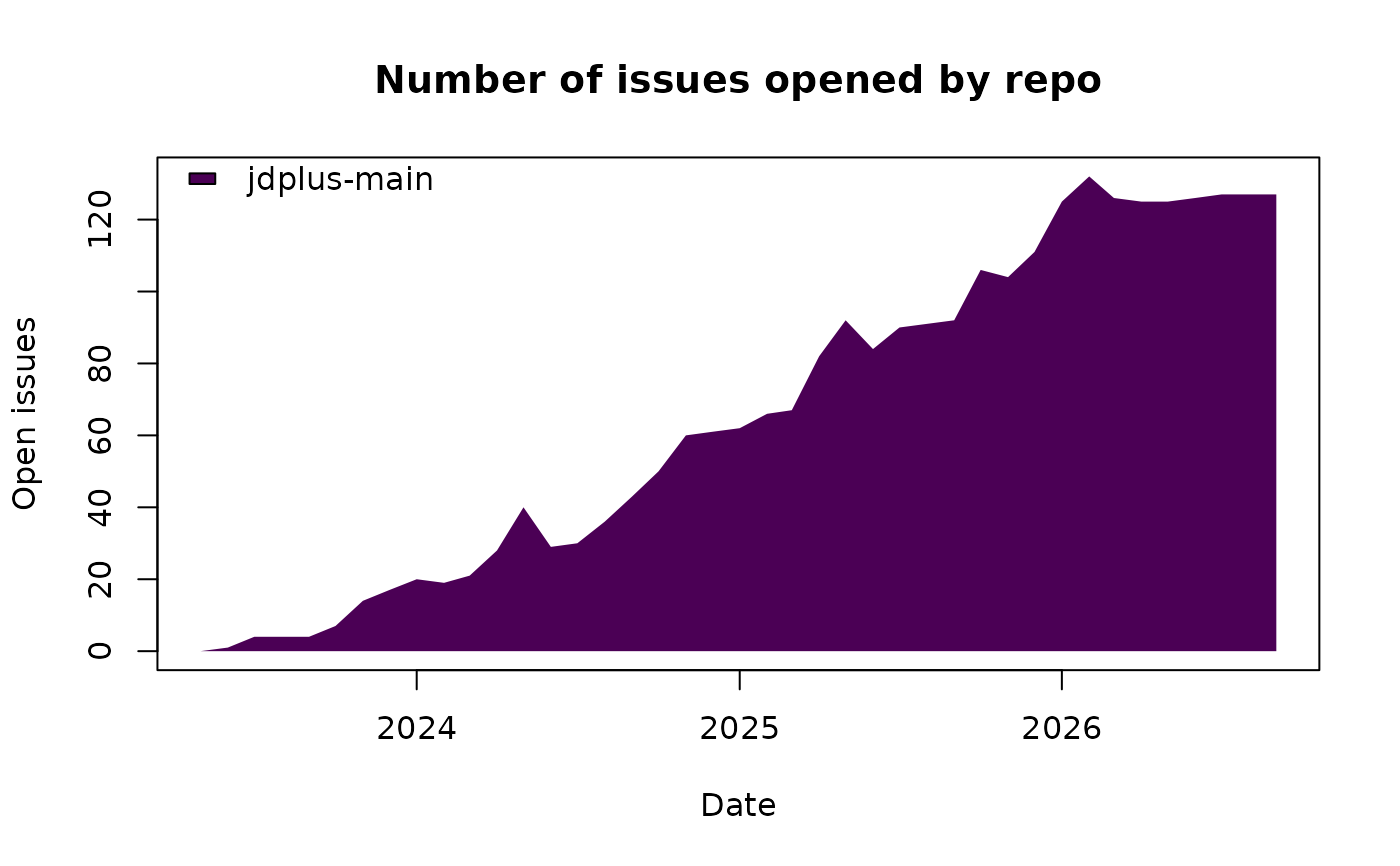
Plot an IssuesTB object — plot-issues • IssueTrackeR

Visualize the evolution of an issue tracker backlog.

Two types of plots are available:

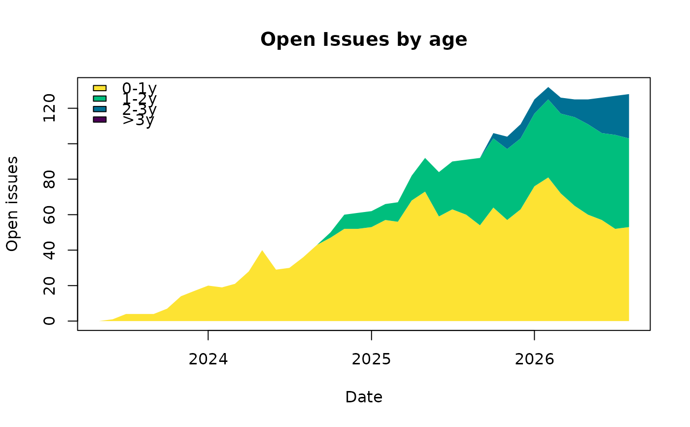
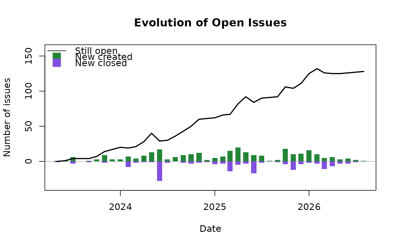
"historic": displays the distribution of open issues by age.
"created-closed": displays backlog size together with the numbers of newly created and newly closed issues.

# S3 method for class 'IssuesTB'
plot(
  x,
  type = c("historic", "author", "created-closed", "resolution-time"),
  n = 3L,
  ...
)

Arguments

x: An object of class IssuesTB.
type: Character string indicating which plot to produce. Accepted values are "historic" and "created-closed". The default is "historic".
n: Integer specifying the number of age classes to display when type = "historic".
...: Currently not used.

Value

Invisibly returns x.

Details

When type = "historic", a stacked area chart is produced showing the number of open issues by age over time. This visualization highlights the evolution and aging of the backlog.

The first classes correspond to one-year intervals (0-1y, 1-2y, ..., (n-1)-ny) and the last class groups all issues older than n years.

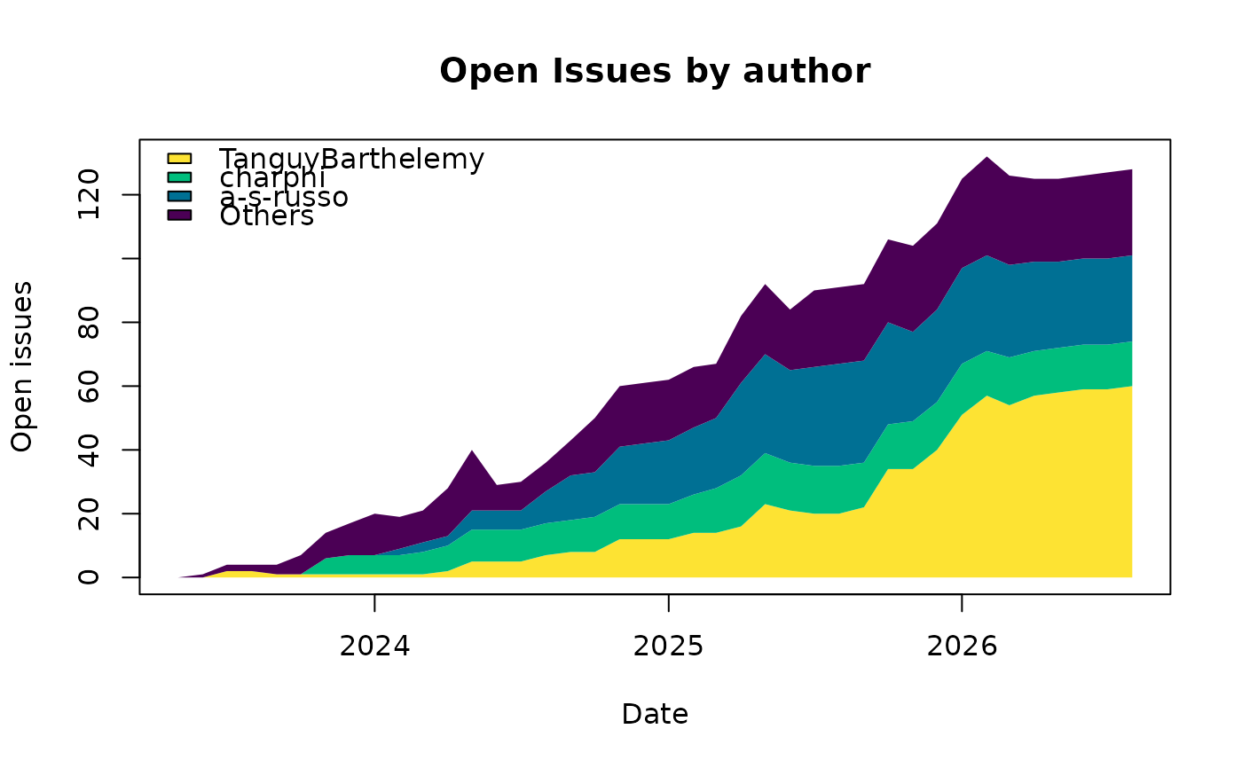
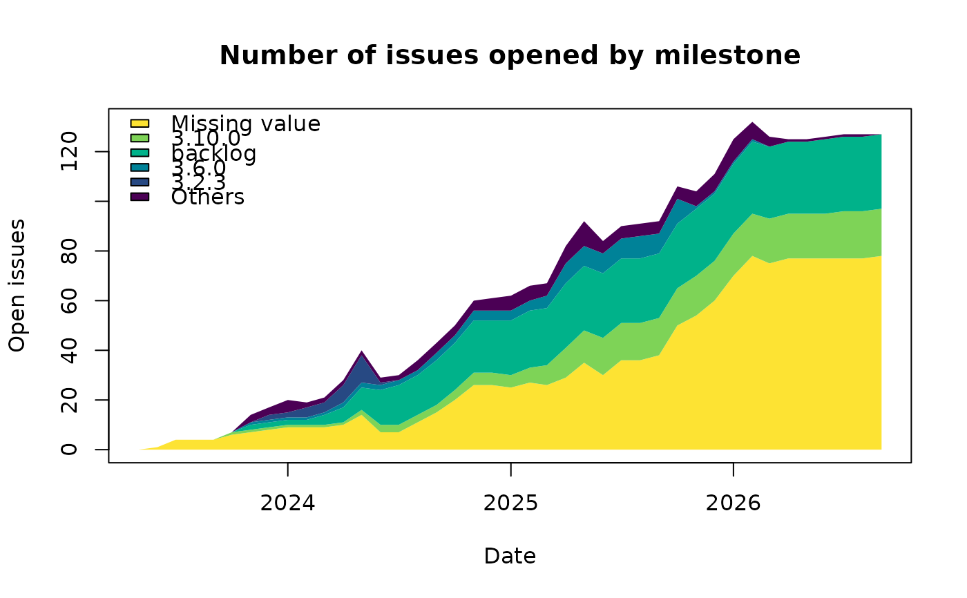
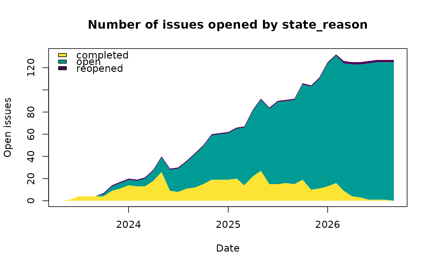
When type = "author", the same graph as type = "historic" but this time with the number of open issues by author over time.

When type = "created-closed", the total number of open issues is displayed together with the monthly numbers of newly created and newly closed issues. This visualization helps assess whether issue creation and resolution rates are balanced over time.

All statistics are aggregated monthly, from the month of the first issue creation to the current date.

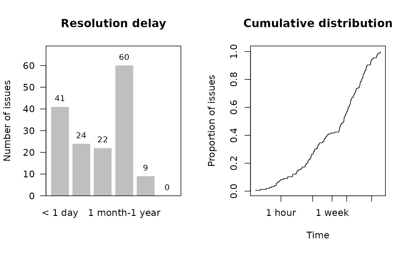
When type = "resolution-time", the resolution times are computed and displayed in two forms:

bar plot with categories from time
ECDF to show the cumulative distribution of issues resolution times on a log scale

Examples

all_issues <- rbind(
    get_issues(
        source = "local",
        dataset_dir = system.file("data_issues", package = "IssueTrackeR"),
        dataset_name = "open_issues.yaml"
    ),
    get_issues(
        source = "local",
        dataset_dir = system.file("data_issues", package = "IssueTrackeR"),
        dataset_name = "closed_issues.yaml"
    )
)
#> Looking into open_issues.yaml ...
#> The issues will be read from /home/runner/work/_temp/Library/IssueTrackeR/data_issues/open_issues.yaml.
#> Looking into closed_issues.yaml ...
#> The issues will be read from /home/runner/work/_temp/Library/IssueTrackeR/data_issues/closed_issues.yaml.

plot(all_issues, type = "historic")

plot(all_issues, type = "author")

plot(all_issues, type = "created-closed")

plot(all_issues, type = "resolution-time")